This blog will provide simple steps allowing the use of a signal generator to create and observe “leakage”, and to apply windows and observe the effects on the frequency spectrum data.
What happens if you do not window a signal? If you have only been doing signal analysis for a short time, you may have accepted that you need to add a window to your signal processing, and understand that the amplitude accuracy is partially improved by turning on a window. However, it can be instructional (and not too difficult) to experiment with a signal generator and an analyzer to see how this affects real world measurements, and why windowing is used to reduce “leakage”, which you would likely observe with almost any signal you measure in a typical analysis application.
The first step would be to connect an output channel on your signal analyzer to one of the input channels. If there is no output channel available, you can use an external signal generator, though it is much easier to use the built in generator.
Open up Data Physics SignalCalc software and choose the Auto Power Spectrum test. Make sure your input channel is not set to ICP, and units are set to Volts (not required, but more accurate for this demonstration). Click on the “Generator” tab, and make one of the generator channels active with a sine wave, level set below the maximum range you current have set for your input.
SignalCalc 730 Channels Table
Generator Tab
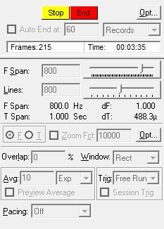
To keep things simple, also go ahead and set your F Span to 800 Hertz, and your Lines to 800 lines, which gives a ?F of exactly 1Hz (not required, but again, easier for this demonstration). Finally, set your windowing to rectangular.
SignalCalc 730 Run Panel
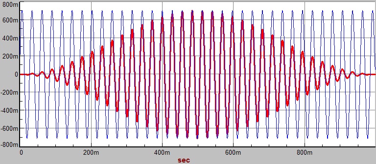
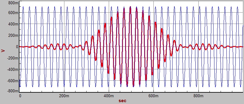
For displays, add a “last Auto Power Spectrum”, “Windowed Time”, and “Last Time History” for the first channel so you can observe what’s happening.
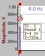
Now simply start the test! If you have the frequency set to 4 Hz, a nice integer multiple, you should see a single frequency line in the auto power spectrum, and your amplitude should match the level you set on the generator tab.
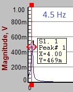
Now you can start adjusting the frequency without stopping the test. Start adjusting the frequency slightly so that it is no longer an integer multiple of the ?F, and you should start to see the leakage appear, and you should start to see your peak amplitude drop down also. It will be quite close to the nominal value when you’re close to an integer multiple of ?F, and you will see the maximum error when you set the frequency to n.5 times ?F. That should be pretty close to the values you have probably seen in tables showing the various errors of different windowing methods.
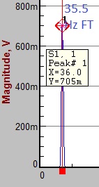
.705V amplitude
.469V amplitude
Now start trying the same thing with different windowing functions, especially the two most common, Hanning and Flattop. You’ll be able to observe the more accurate amplitude accuracy of these two windows, and you should see the shape of the windows in the “Windowed Time” display.
Now start trying the same thing with different windowing functions, especially the two most common, Hanning and Flattop. You’ll be able to observe the more accurate amplitude accuracy of these two windows, and you should see the shape of the windows in the “Windowed Time” display.
Hann Window function
Amplitude is much closer here.
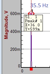
Flattop Window Function
Almost no error in amplitude at 35.5 Hz with Flat Top Window
You can continue to try different combinations of frequencies windows to answer questions that may have occurred to you. (One great trick with SignalCalc is that if you set your generator frequency to a negative value, it will generate precisely that number of cycles within the time window you are observing, so if you select -10, it will create exactly 10 cycles in the data.)
This is also a great way to see what nominal measurements of other types of signals such as random, saw tooth, square waves, etcetera, look like in the frequency domain and with windows applied. The nice thing about this method is that it takes very little time and can show you a bit more directly how your data is impacted in a real sense, rather than in a theoretical sense. This can later make the equations easier to understand as you develop your expertise in signal processing.
