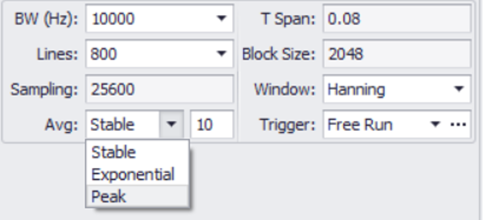
Spectral averaging can help alleviate noise and moment-to-moment fluctuations seen often in instantaneous measurements, and as such it is standard practice to use spectral averaging when characterizing certain vibration environments. SignalCalc 900’s Autopower Spectrum Module has three distinct averaging techniques, Stable, Exponential, and Peak. It is important to understand these averaging techniques and their strengths and weaknesses to help determine the most appropriate selection for a specific test.
SignalCalc 900 Averaging Selections
Stable (Linear) Averaging
The Stable selection sums a preset number of results, weighting each with equal importance. During acquisition, the average is automatically normalized to the number of frames currently acquired. The numerical entry window represents the number of frames to be averaged. Individual frame durations are equal to the TSpan parameter, which is determined based on the FFT acquisition settings (Bandwidth and Lines).
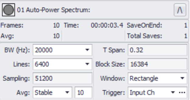
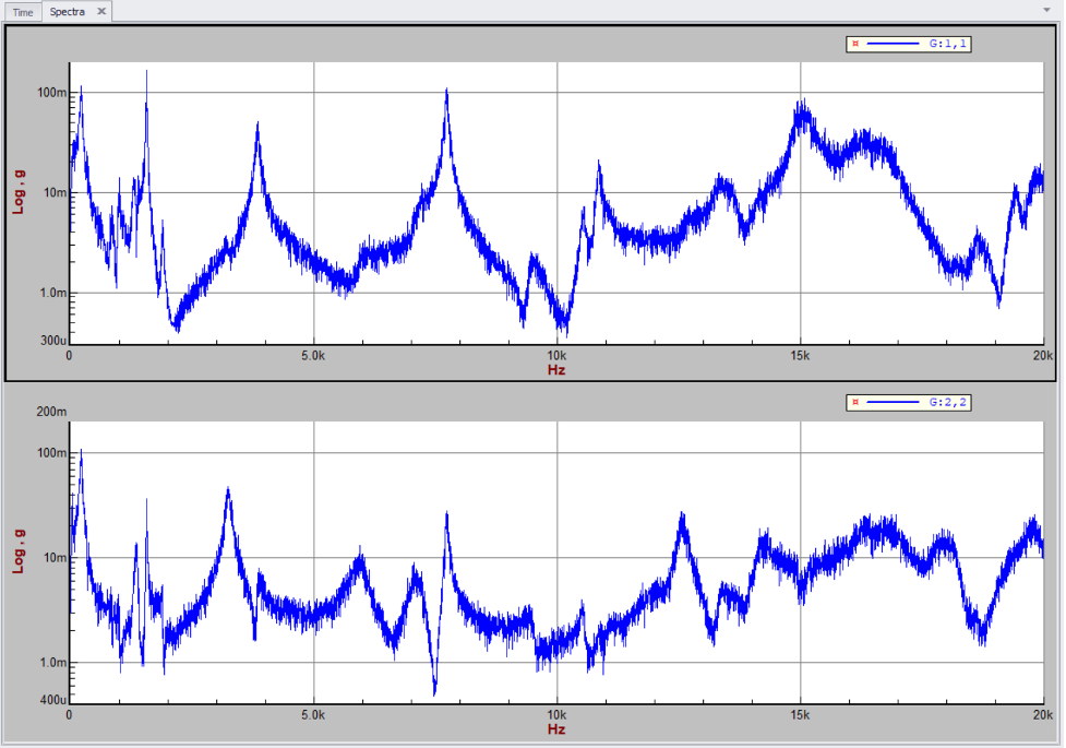
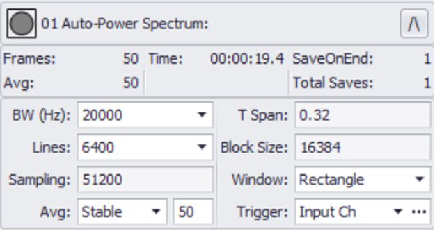
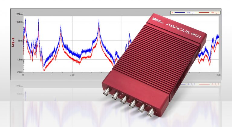
The higher number of averages selected, the lower the effect of noise will be. See below, a response measurement on a structure (driven by a Random signal) with 10 averages, and again with 50 averages.
SignalCalc 900 APS Random, Stable 10
SignalCalc 900 APS Random, Stable 50
Exponential Averaging
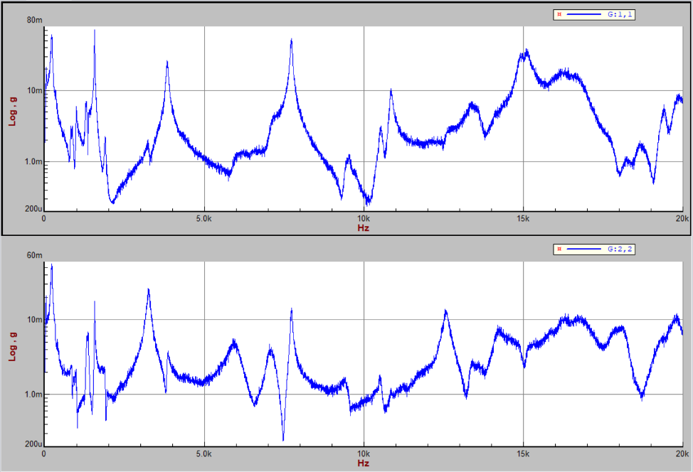
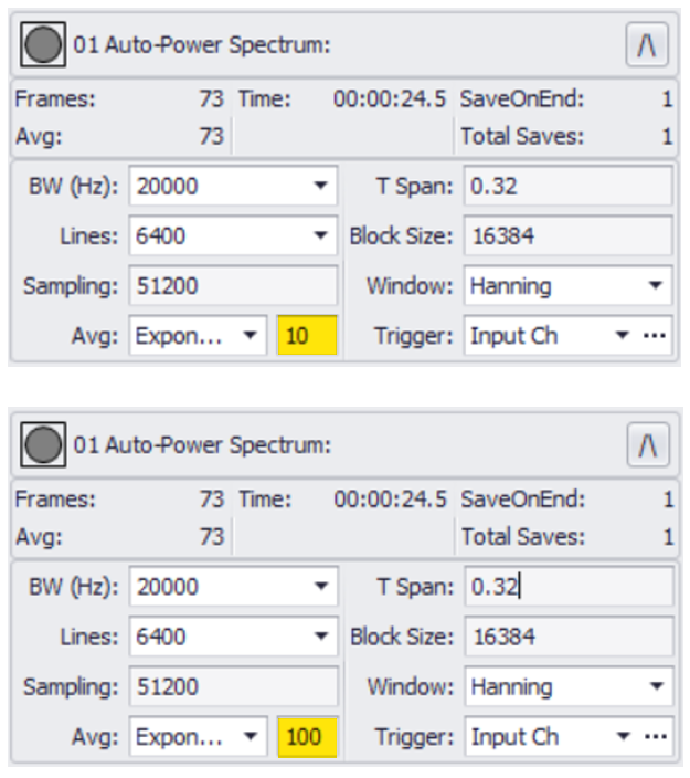
Exponential selection provides a time-weighted moving average that continues from the time the Start button is pressed, until the Stop button is pressed. The current frame is weighted most heavily and the influence of older snapshots decays away exponentially with time. This type of averaging is analogous to analog RC smoothing, where the Averages parameter determines the exponential time-constant. It provides a similar signal-to-noise enhancement to like-valued stable averaging with the advantage that time-variant phenomena may be monitored more easily.
The numeric entry can be thought of as the number of T Span intervals in the time-constant. Increasing this value applies less weight to more recent samples (lower number, more sensitive to change).
Current Frame weighted more heavily with settings on the top.
Stable vs Exponential: When to choose what?
Stable averaging assigns equal weighting to all frames, new and old. Such linear weighting is useful for accurate measurements over a specified time interval but not useful when looking for a more “real-time” view of the spectral energy content. More recently acquired data can remain hidden in the Stable Average even if it is large in amplitude This effect is more pronounced when the number of previous frames is large. Conversely, the Exponential average selection, applies a greater weight to more recent samples, and runs continuously until the user triggers a stop. When dealing with a constrained or pre-defined time interval, Stable averaging may be a more appropriate option. When recent data is more important than previous data, Exponential may be the most appropriate option. Exponential averaging provides more of a “Real-time” view while Stable provides a traditional “Average” view.
Peak Averaging
The Peak selection is not a traditional averaging process. In this mode, the maximum value encountered at each frequency point in each frame is retained. That is, a “roof extrema” or “envelope” is retained. The numerical entry window determines the number of frames to hold maximum values across. This selection is useful for determining the maximum magnitudes that occurred at each frequency, regardless of which frame they occurred during. An example of this selection is given below. Notice the difference in the peak magnitudes compared to the Stable and Peak selections.